Numpy basics
Posted on March 8, 2019 at 12:00 PM

In this tutorial we take a look at the basic features of the Python package NumPy. NumPy is an essential package for data science tool kits and well worth taking the time to learn.
What is NumPy?
Numpy is a library used for scientific computing. In a nutshell it can compute using arrays much faster and simply than a doing the same operation with a python list.
Installing NumPy
NumPy is not installed by default and thus must be installed using pip:
pip install numpy
NumPy basics
Once installed, you must import NumPy; the convention is to "import numpy as np" as depicted below. After that can create an array by passing in a list of values. In this case, we are looking at some made up data for height and weight to compute BMI. Note, when adding lists together, the add works like concatenation. With a NumPy array, the respective numbers are added together from the two arrays.
>>> import numpy as np
>>>
>>> height = [1.73, 1.68, 1.71, 1.89, 1.79]
>>> weight = [65.4, 59.2, 63.6, 88.4, 68.7]
>>>
>>> np_height = np.array(height)
>>> np_weight = np.array(weight)
>>>
>>> bmi = np_weight / np_height ** 2
>>> bmi
array([21.85171573, 20.97505669, 21.75028214, 24.7473475 , 21.44127836])
>>>
>>> height + height
[1.73, 1.68, 1.71, 1.89, 1.79, 1.73, 1.68, 1.71, 1.89, 1.79]
>>>
>>> np_height + np_height
array([3.46, 3.36, 3.42, 3.78, 3.58])
Subsetting/ slicing arrays
As with a python list you can slice based upon a index number. You can also apply logic which returns an array of Booleans, or slice with the logic.
>>> bmi
array([21.85171573, 20.97505669, 21.75028214, 24.7473475 , 21.44127836])
>>>
>>> bmi[0]
21.85171572722109
>>>
>>> bmi > 23
array([False, False, False,  True, False])
>>>
>>> bmi[bmi > 23]
array([24.7473475])
>>>
2 dimensional arrays
You can have 2 dimensional NumPy arrays. Calling the "shape" attribute shows how the array is structured (in this case 2 rows and 5 columns). You can also slice 2d arrays as with a 1d array; array[row, column]
.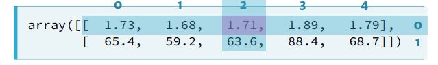
>>> np_2d = np.array([[1.73, 1.68, 1.71, 1.89, 1.79],
 [65.4, 59.2, 63.6, 88.4, 68.7]])
>>> np_2d
array([[ 1.73,  1.68,  1.71,  1.89,  1.79],
       [65.4 , 59.2 , 63.6 , 88.4 , 68.7 ]])
>>>
>>> np_2d.shape
(2, 5)
>>>
>>> np_2d[0]
array([1.73, 1.68, 1.71, 1.89, 1.79])
>>>
>>> np_2d[0][2]
1.71
>>>
>>> np_2d[0,2] # this is a preferable way to slice although the line above also works
1.71
>>>
>>> np_2d[:,1:3]
array([[ 1.68,  1.71],
       [59.2 , 63.6 ]])
>>>
Note, you cannot store two different types of data in an array; one data type will be converted to match the other. Take a look at the following example where the integers are converted to strings:
>>> test = np.array([[1,2,3],['a','b','c']])
>>> test
array([['1', '2', '3'],
       ['a', 'b', 'c']], dtype="")
Boolean operators
You can also do more complex queries using Boolean operators. Typically in Python you will see an equation that may look like this:
>>> x = 10
>>> x > 5 and x < 15
True
>>>
When using a NumPy array you must use:
- logical_and()
- logical_or()
- logical_not()
>>> np.logical_and(np_2d > 1.8, np_2d < 80)
array([[False, False, False,  True, False],
       [ True,  True,  True, False,  True]])
>>>
>>> np_2d[np.logical_and(np_2d > 1.8, np_2d < 80)]
array([ 1.89, 65.4 , 59.2 , 63.6 , 68.7 ])
>>>
Basic statistical analysis
The main use of NumPy is to do statistical analysis across big data sets. For this example, I have generated some random data to use (symbolising height and weight) across a sample of 5000. We can then analysis things like the sum, mean, mode, standard deviation, correlation and much more. In this example, we take a slice to get all the heights and subsequently work out the mean, median, correlation and standard deviation.
>>> height = np.round(np.random.normal(1.75, 0.20, 5000), 2)# distribution mean, distribution standard deviation, number of samples
>>> weight = np.round(np.random.normal(60.32, 15, 5000), 2)
>>> np_city = np.column_stack((height, weight)) # merge the two data sets together
>>>
>>> np.mean(np_city[:,0])# this slice gets all the rows for the height column
1.751134
>>>
>>> np.median(np_city[:,0])
1.75
>>>
>>> np.corrcoef(np_city[:,0], np_city[:,1])
array([[1.        , 0.00718604],
       [0.00718604, 1.        ]])
>>>
>>> np.std(np_city[:,0])
0.19722589597717638
>>>
dir(np_city)
Don't forget you can always use built in functions like help(), dir() and type() as these are useful to work out what else you can do with your data. Notice, the additional functions like sum, min, max which are useful ways to check out your data
>>> dir(np_city)
['T', '__abs__', '__add__', '__and__', '__array__', '__array_finalize__', '__array_interface__', '__array_prepare__', '__array_priority__', '__array_struct__', '__array_ufunc__', '__array_wrap__', '__bool__', '__class__', '__complex__', '__contains__', '__copy__', '__deepcopy__', '__delattr__', '__delitem__', '__dir__', '__divmod__', '__doc__', '__eq__', '__float__', '__floordiv__', '__format__', '__ge__', '__getattribute__', '__getitem__', '__gt__', '__hash__', '__iadd__', '__iand__', '__ifloordiv__', '__ilshift__', '__imatmul__', '__imod__', '__imul__', '__index__', '__init__', '__init_subclass__', '__int__', '__invert__', '__ior__', '__ipow__', '__irshift__', '__isub__', '__iter__', '__itruediv__', '__ixor__', '__le__', '__len__', '__lshift__', '__lt__', '__matmul__', '__mod__', '__mul__', '__ne__', '__neg__', '__new__', '__or__', '__pos__', '__pow__', '__radd__', '__rand__', '__rdivmod__', '__reduce__', '__reduce_ex__', '__repr__', '__rfloordiv__', '__rlshift__', '__rmatmul__', '__rmod__', '__rmul__', '__ror__', '__rpow__', '__rrshift__', '__rshift__', '__rsub__', '__rtruediv__', '__rxor__', '__setattr__', '__setitem__', '__setstate__', '__sizeof__', '__str__', '__sub__', '__subclasshook__', '__truediv__', '__xor__', 'all', 'any', 'argmax', 'argmin', 'argpartition', 'argsort', 'astype', 'base', 'byteswap', 'choose', 'clip', 'compress', 'conj', 'conjugate', 'copy', 'ctypes', 'cumprod', 'cumsum', 'data', 'diagonal', 'dot', 'dtype', 'dump', 'dumps', 'fill', 'flags', 'flat', 'flatten', 'getfield', 'imag', 'item', 'itemset', 'itemsize', 'max', 'mean', 'min', 'nbytes', 'ndim', 'newbyteorder', 'nonzero', 'partition', 'prod', 'ptp', 'put', 'ravel', 'real', 'repeat', 'reshape', 'resize', 'round', 'searchsorted', 'setfield', 'setflags', 'shape', 'size', 'sort', 'squeeze', 'std', 'strides', 'sum', 'swapaxes', 'take', 'tobytes', 'tofile', 'tolist', 'tostring', 'trace', 'transpose', 'var', 'view']
>>>
Its worth also point out that you can loop through arrays as you would also data types in Python, but if you find yourself doing this, you may want to check this is the correct thing to be doing.
Code takeaway
import numpy as np
height = [1.73, 1.68, 1.71, 1.89, 1.79]
weight = [65.4, 59.2, 63.6, 88.4, 68.7]

np_height = np.array(height)
np_weight = np.array(weight)

bmi = np_weight / np_height ** 2

x = bmi>23
print(x)
print(type(x))


print(bmi)
print(bmi[0])
print(bmi > 23)

print(bmi[bmi > 23])

np_2d = np.array([[1.73, 1.68, 1.71, 1.89, 1.79],[65.4, 59.2, 63.6, 88.4, 68.7]])
print(np_2d)

print(np_2d.shape)
print(np_2d[0])
print(np_2d[0][2])
print(np_2d[0,2])
print(np_2d[:,1:3])


height = np.round(np.random.normal(1.75, 0.20, 5000), 2)# distribution mean, distribution standard deviation, number of samples
weight = np.round(np.random.normal(60.32, 15, 5000), 2)
np_city = np.column_stack((height, weight)) # merge the two data sets together

print(np.mean(np_city[:,0]))# this slice gets all the rows for the height column
print(np.median(np_city[:,0]))
print(np.corrcoef(np_city[:,0], np_city[:,1]))
print(np.std(np_city[:,0]))

print(dir(np_city))
import numpy as np height = [1.73, 1.68, 1.71, 1.89, 1.79] weight = [65.4, 59.2, 63.6, 88.4, 68.7] np_height = np.array(height) np_weight = np.array(weight) bmi = np_weight / np_height ** 2 x = bmi>23 print(x) print(type(x)) print(bmi) print(bmi[0]) print(bmi > 23) print(bmi[bmi > 23]) np_2d = np.array([[1.73, 1.68, 1.71, 1.89, 1.79],[65.4, 59.2, 63.6, 88.4, 68.7]]) print(np_2d) print(np_2d.shape) print(np_2d[0]) print(np_2d[0][2]) print(np_2d[0,2]) print(np_2d[:,1:3]) height = np.round(np.random.normal(1.75, 0.20, 5000), 2)# distribution mean, distribution standard deviation, number of samples weight = np.round(np.random.normal(60.32, 15, 5000), 2) np_city = np.column_stack((height, weight)) # merge the two data sets together print(np.mean(np_city[:,0]))# this slice gets all the rows for the height column print(np.median(np_city[:,0])) print(np.corrcoef(np_city[:,0], np_city[:,1])) print(np.std(np_city[:,0])) print(dir(np_city))